A central component of Raynet One is the job graph. It displays the performed job operations in great detail. It differentiates between successful and failed jobs very easily. It is designed to promote the transparency of operations. Inspect it to gain feedback about how your triggered jobs impact the platform and IT landscape health. It encourages the user to build trust in working procedures on display. It is exciting to trace the job's live path of execution, sometimes at least.
In this chapter, we want to describe the components of the job graph user interface. You will learn how to work with it efficiently.
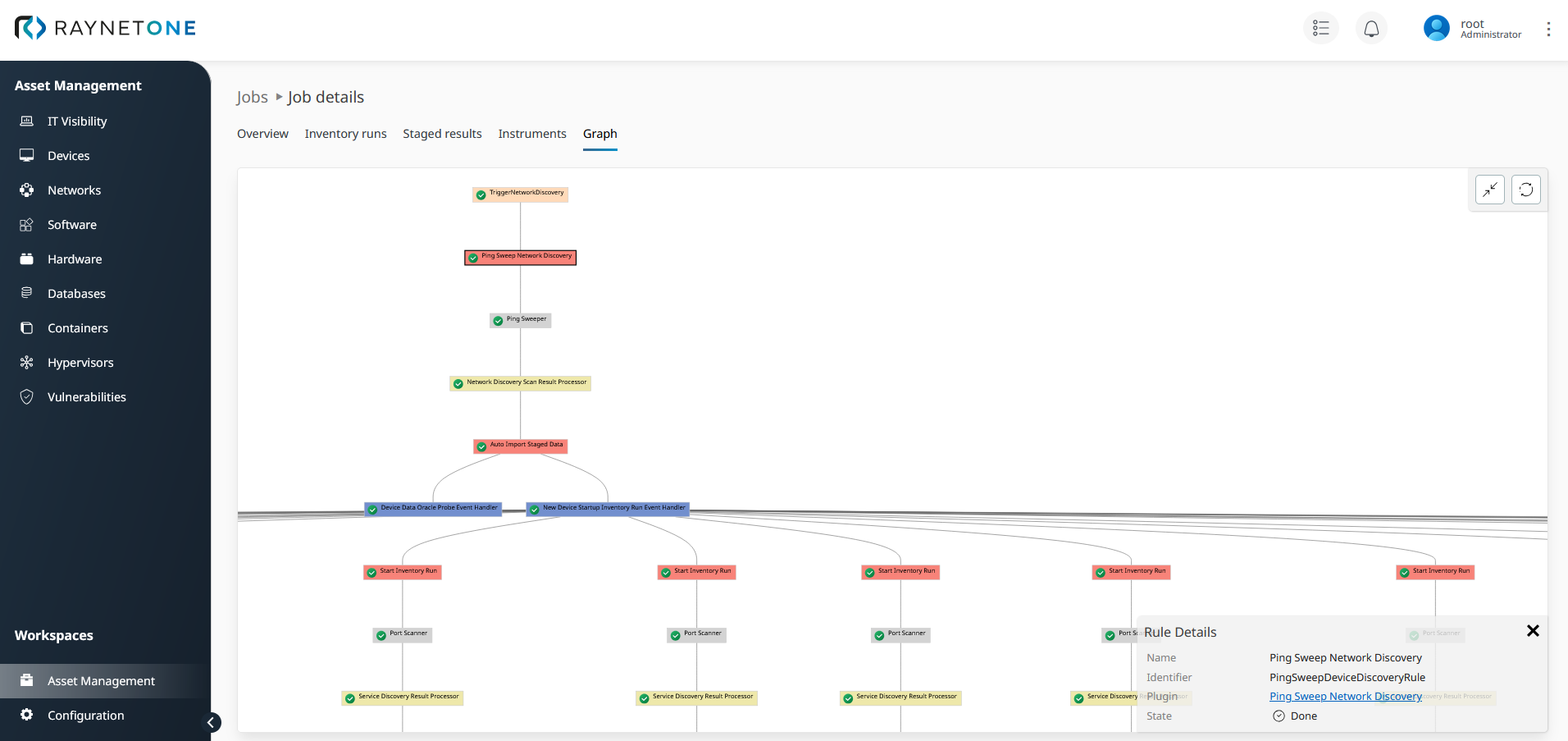
The job graph of a finished network discovery and inventory job. The root node is labeled TriggerNetworkDiscovery. The path below it computes the set of discoverable devices by probing all available network addresses. The gray node is labeled Ping Sweeper. It represents the discovery workload executed on the runner. The red nodes with the text Start inventory run are triggered by the finished discovery task as the platform is configured to automatically inventory newly found devices. In the top right of the graph view you can see two buttons to control the graph view. At the bottom right you can see details of the node selected by left-click.
Moving the graph view
As your mouse is moving over the graph view panel, the mouse cursor turns into an arrow-cross shape.
![]()
The exact icon may be different depending on the web browser or operating system involved. Left-click and drag the mouse to change the graph view-port location.
Zooming the graph view
Just as easily as you can move the graph view, zoom it using your mouse wheel. The mouse cursor has to be on the graph view panel, not on the node description panel. There is a minimum and maximum zoom level.
Job graph control buttons
You can find control buttons at the top right of the view.
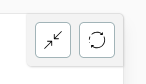
The left button is used to center the graph view to the entire graph. Use it to get a good overview of the graph's structure. Return to a valid graph view in case the graph view-port has gone ways and you are left with a white panel.
The right button is used to refresh the displayed graph to the latest state. The graph does not update automatically to save CPU and bandwidth load.
Node description panel
Valuable information about selected nodes is found in the panel at the bottom right of the view.
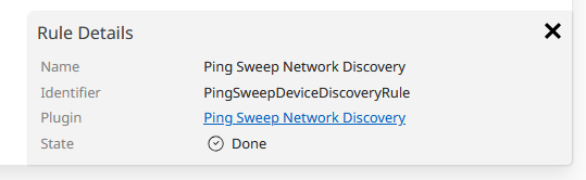
In the above picture, you can see the details of a selected rule node, having the red color. The type of information displayed is bound to the node type and state. Successful nodes have less troubleshooting information to report than failed ones. Let's compare the display in case of failure and success.
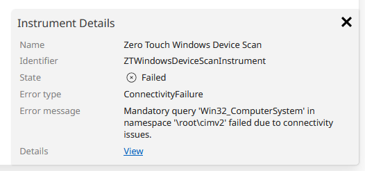
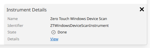
In the two pictures above, you see the details of two instrument execution nodes, the nodes colored gray. This comparison is a good example because the node type is the same but the success state is not. The failed node displays the additional parameters Error type and Error message, designed for a simple visual troubleshooting experience.